All | Optimization

February 20, 2016mgric

Network of Mediciation Side Effects

<br />

I recently stumbled upon a database[1] of prescription and generic medicine that contains all of the side effects listed on thier labels. As we all know from all of those prescription medication commercials (looking at you cialis) the side effects take up about half the commercial. I wondered if certain side effects always showed up together. Kinda how cough and cold are always packaged together. I downloaded and scrubbed the database. From there I broke it up into two groups, the map above and the map below.

The network above has all of the most LIKELY side effects from the medication. This was defined as occurring more than 60% of the time in people who took the medication. This narrowed the 200+ side effects to under 100. I with my very rudimentary medical training grouped these effects into certain categories (bones, blood based, mental, etc). The stroke width of the bonds between two side effects are determined by how many times they both show up together on a side effects list. I created the force graph in d3 with help from two great sources [2][3]. You can manipulate this web and if you double click a point it highlights its neighbors that it is usually paired with.

The network below is the top 50 most COMMON side effects. These side effects appeared most on the labels of all the prescription meds. Because these side effects were so frequent they were connected to everything and produced a rather boring glob of points (as you can see below now). I further restricted the bonds by only keeping links that appeared over 200 times. This produced a (slightly) less intricate web. You can move the slider to break and form bonds, weaker bonds break first. This network also allows for double clicking.

Pretty cool stuff. This might be useful for prediction as certain side effects are always linked together. Future steps might be a more rigorous grouping rather than my less-than informed medical opinion.

All the visualization credit goes to the bottom two sources. All the above is based of the work of the two below. They helped me immensely as I am a novice in javascript. Also a quick shoutout to the [4] source as it was a complete pain to get d3 working with wordpress.

-Marcello

[1]http://sideeffects.embl.de/

[2]https://bl.ocks.org/mbostock/4062045

[3] http://www.coppelia.io/2014/07/an-a-to-z-of-extra-features-for-the-d3-force-layout/

[4]https://www.datamaplab.com/posts/embedding-javascript-visualization-wordpress/

January 15, 2016mgric

Journal Club: Week of 1/15/16

Graphical Perception: Theory, Experimentation, and Application to the Development of Graphical Methods

William S. Cleveland; Robert McGill

Journal of the American Statistical Association

This paper is a little different from the previous papers I’ve read. It does not outline new optimization methods or review machine learning algorithms. This paper just looks out how we display data, which has become a huge field in the most recent years. Cleveland and McGill wrote this paper before the wave of data analysts and data scientists, back in 1984. However, there findings are still very relevant and super useful.

The paper outlines a study on perception. The authors sought to determine which charts and graphs are the most easily interpret-able and most accurate. They broke down the interpretation and structure of graphs into 10 “elementary perceptual tasks” which describe features that graphs use to separate data. The ten tasks are as follows ranked in best to worst:

1.position along a common scale

2. position along non aligned scales

3. Length, Direction, Angle

4. Area

5. volume, curvature

6. shading, color saturation

This is quite an interesting list especially when looked at in terms of todays graphical documents. One of my favorite visualizations is the cholorpleth maps which rely almost entirely on color saturation, however this task fared the worst! Keeping these tasks in mind the authors iterate through common graphs. Some scored better than others, Bar charts topped most of their tests, while the widely hated pie chart scored toward the bottom.

This paper is full of graphs and charts to show their findings and examples of how some graphs fail and other succeed. A particularly interesting example is the distance between two curves. On the left the show a matrix of two curves and asked their participants to estimate the distance between the two curves at various points. On the right is the actual difference of the two curves. I found that even after reading the paper I would stumble on my perception of the two curves.

This paper is excellent. I highly suggest that anyone who makes graphs gives it a quick read. The graphs look a little dated, but nevertheless contain tons of information. It even has some recommendations on common graphs to replace with graphs that better display information.
One thing the paper does not capture is the recent trend to make graphs as pretty as possible. There is an obvious trade off that the creator must decode. Do I want to make a pretty graph that entices clicks or a utilitarian graph which conveys the most amount of information? Reading this paper brings us a little closer to a happy compromise.

January 12, 2016mgric

Follow The Money

Campaign finances are becoming a prominent issue in today’s elections. We have candidates like Jeb Bush who are receiving record breaking amounts of donations from private citizens and private companies alike. On the other hand we have candidates like Bernie Sanders who only receives small donations from citizens. Regardless of your opinion on which end of the spectrum candidates should behave toward campaign donations, they are nevertheless an important part of US elections. When discussing campaign donations it is almost always about presidential candidates, but what about our legislators. They only time I ever heard about donations to legislators is when there is a huge scandal. Do they pull in as much money as presidential candidates? Do they receive more money from the average citizen or the average corporation? Do legislators of a certain party pull in more than another?

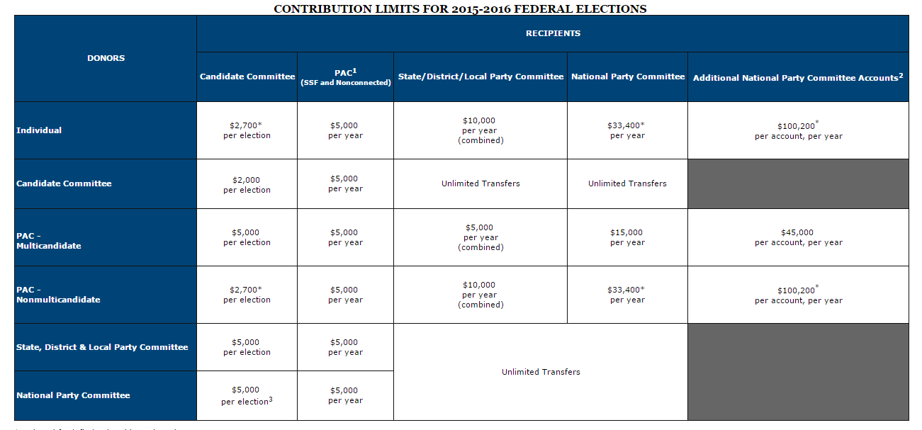
To achieve this I needed data on campaign donations for all the federal legislators. Luckily for me I am not the first to look for this data. There are quite a few places to go to for this information, but I wanted a place with an easy to understand API and something reliable. This led me to followthemoney.org. Here there is a very soft “API”, but nevertheless super useful and easy to parse. I took the data for all legislators from the past 5 years for any candidate that ran for either the Senate or the House of Representatives. Using their API, I exported their data in csv format. From there the preprocessing and the analysis was all preformed in python (anaconda distribution).

Before we jump into the analysis we need to know a little more about campaign contributions themselves. There are federal contribution limits imposed to limit how much people (and corporations, parties, PACS, etc..) can donate. There are a few ways to get around these limits however and recent legislature that has helped to facilitate that.

The two recent major decisions that we need to know for analysis are McCutcheon v. FEC and Citizens united v. FEC. Both of these decisions deal with how much people can contribute to candidates. Citizens United v. FEC[1] prohibited the government from restricting political expenditures by a non-profit organization. This however is subtly different than direct campaign donations, this type of expenditure[2] endorses the candidate but is made independently from the candidate. This we have to keep in mind when discussing PACs, as this is a heavily used tactic to funnel large sums of money into a candidate. The other decision was McCutcheon v. FEC[3], this decision removed the aggregate limits on campaign contributions. These decisions have brought in new spending and new ways to spend. It is more important

STATE OF THE UNION

Now that we know who can donate and how much they can donate, let’s see who is on the receiving end. One more important thing we need to know is when all of our candidates are up for election. As we all know Senators serve a total of six years, with 1/3 of the Senate up for reelection every two years. Congressmen on the other hand only serve two years and are up for election every two years. Elections fall on the even numbered years, so our important data will fall on 2010, 2012, and 2014. All other years are reserved for special elections, like if a senator dies midterm. For this first part I am using the data from the 2014 elections.

In 2014, the average Senator/Congressman pulled in a little over a million dollars in campaign donations. This average is a little skewed as some legislators pulled under a thousand and some over 10 million. The range of the campaign donations is set by these two men, Mitch McConnell and John Patrick Devine. Mitch McConnel, a republican and more importantly the Majority leader of the Senate, pulled in a whooping $30 million, while John Patrick (whose googling revealed no pertinent results) pulled in a less than stellar $40. Naturally, John Patrick lost his race, while Mitch McConnel is our current majority leader and has held his office in the senate since 1985.

Speaking of winners and losers, who makes more? Naturally, I believe that the average winner should pull in a great deal more than the average loser. And well, that’s pretty much how it goes. Winners bring in an average of $2 million while losers can only muster up about half a mill. This is however, excluding a group of politicians who chose to withdraw from the race. Looking at those politicians they close the gap, but not by much they pull in half of that as winner, $1 million.

Before we dive into state by state trends lets see how the Senate do against the house of reps. Below the graph sums up this subsection.

The House pulls in a lot more donations than the Senate. However, this may be due to the sheer amount of people that run for the House. This brings us to a good point. Donations are heavily influenced by the amount of people who run and the amount of people who donate. To avoid making everything based simply on population rather than underlying trends. Most of the following graphs will be averages or per capita when necessary.

Keeping that in mind, let’s see how all 50 states line up. Below is a graph on donations per capita.

2014 Camaign Donations to Legislators Grand Total

That’s much better. As you can see this is obviously not a population map. States like NY, NJ, MA, and CA are not top tier, but rather toward the bottom. Interestingly enough, states that have less people in them seem to have much greater donations per person, Alaska is a notable example. Why do these states get way more contributions than others? One possible explanation are that some of theses states are swing states. Swing states (like New Hampshire above) are very closely divided between the Republicans and the Democrats. These states should naturally garnish more donations as the races should be more exciting and volatile. In coarser terms, campaign money is more valuable in these states.

Before we go any further, we have to go into whose donating, lets take a look nationwide as to who is donating the most. Is it mostly large sums, or small donations?

PEOPLE, PACS, AND THINGS

Speaking of small donations, who actually donates to campaigns? I personally have never, my naïve and uninformed idea of campaign donations are just giant faceless corporations throwing money at candidates. Let’s take a peek at average joes like you and me and how much they spend. Below you can see two maps of the US, one for 2012 and one for 2014. Hover over each state to see which citizen donated the most and how much they donated, the color scale lets you compare states to each other.

These two maps display the top donators for each state in 2012 and 2014. As you can see in 2012 Texas and Connecticut dominated in terms of individual donators. These points may have skewed the data however, as Linda from Connecticut was actually running in the campaign herself, personally funding her run. David from Texas was the lieutenant governor of Texas during that time. These do not seem like ordinary people.

2014 paints a more familiar (and relate-able) campaign. The donations are much lower than in 2012, but similar trends emerge. New York, California and Texas are all toward the top in terms of individual donators. With “fly-over” states toward the bottom.

Now what about those big faceless corporations. Here are two more maps, however these are only for the year 2014. The map on the left shows the the top Industry for that state the chart on the right shows the top ten Industries that donate the most nationwide.

Again we have what looks to be a population map. It seems like states with the most people have the highest individual donators whether from citizens or corporations. One thing that stood out to me were the biggest donors. Real estate and medical professionals we the top players in most states. Much less surprising was that Oil & Gas donated the most where, you guessed it, there is Oil & Gas.

Finally, what about groups who donate based on different ideology? Some examples of these groups are pro-Israel, Pro-Life/Pro-Choice, environmental policy as well as many others. The bar chart on the left shows a nationwide average of which ideologies get the most money. The map on the left shows the most popular ideology per state.

Unfortunately the way followthemoney.org structures its data makes looking at ideologies a little boring. General Liberal and Conservative ideologies are grouped. Obviously these dominate nationwide. However, there are some other ideologies that creep up after these two power houses. Big issues like Foreign policy and environment garner some money. These ideologies do not nearly donate as much as some of the smaller industries. Excluding Liberal and Conservative, ideologies donate ten fold less than industries.

PARTY FOUL

So far we have skipped over the two most important groups in American politics, the Republicans and the Democrats. How do the parties compare? Seeing that the country is pretty divided on party allegiance I’d expect donations to each party be relatively the same. One thing I’d also expect is that third party candidates don’t pull in even the same magnitude as the two major parties.

Well that seems about right. Democrats and Republicans pull in around the same amount each year, while third party candidates are not even close. This was to be expected as third-party candidates rarely have the same pull nor presence as candidates from the two major parties.

Now what about statewide. During presidential elections most states are glazed over. This is because they are usually deeply entrenched in one party of the other. Below is a map of which party got each states electoral votes. Next to that is which party got more money in the 2014 elections.

from: Politico.com

The first graph from Politico shows which party each state voted for. The one below is which party received more donation in each state. The two maps look quite similar. Both the east and west coast mirror each other to an extent. The midwest also aligns with donations. Donations to legislators in each state may be a good predictor into where the electoral votes end up. Or, more possibly, states that were going to vote for a certain party donate to that party more.

Some states receive a lot more attention than other when it comes time for presidential elections. Currently I am only looking at federal legislator’s donations, but I wonder if they reflect presidential politics as well. Certain states I will refer to as swing states. These states are not as deeply entrenched as others. The swing states for 2014 were: Nevada, Colorado, Iowa, Wisconsin, Ohio, New Hampshire, Virginia, North Carolina, and Florida. The map below highlights states that have the closest spending between the Democrats and the Republicans.

Most of the swing states have very similar donations between the two parties. Swing states like Virginia, Florida, and Nevada have very close donations totals. Virginia actually has the closest out of all of the states. On the other end, states like California, Texas, and New York have the greatest difference in donations. This makes sense as these states are deeply entrenched in one party, just look at Texas the donations are completely lopsided. There is some good news in this map. Most states are relatively close when it comes to donations to both parties.

MONEY MONEY MONEY MONEY

Political Donations are a critical component of the United States government. Looking at the donations many of my previous assumptions were confirmed and many were discredited. However, one must have a critical eye on the data presented. The analysis is only as good as the data collected. I believe it is integral to have reliable and vetted donation data as it holds many insights. I’d like to thank followthemoney.org for their data and commitment. If you liked this analysis please check out their website and explore the data yourself! Maybe even consider donating!

-Marcello

[1] https://en.wikipedia.org/wiki/Citizens_United_v._FEC

[2] https://en.wikipedia.org/wiki/Independent_expenditure

[3] https://en.wikipedia.org/wiki/McCutcheon_v._FEC

December 4, 2015mgric

Journal Club: Week of 12/4/2015

A Few Useful Things to Know about Machine Learning
Pedro Domingos
Department of Computer science and Engineering University of Washington

This was an excellent read. I highly suggest this paper to novices and expert alike. Pedro goes through all the mysticism and what he calls “folk knowledge” in this paper. Knowledge that would takes years of machine learning you uncover. Pedro breaks down machine learning to simple concepts and shows the reader how to deal with them. Do not be mistaken, this is not a tutorial. You will not learn any new algorithms or application. You will only learn how to better use the ones you know. That being said, I believe it is best to go into this paper with a little background so you are not lost by what Pedro is explaining.

Pedro explores major pitfalls of people who are first learning machine learning as well as seasoned pros. I particularly liked his section on overfitting and the section on how to approach problems. ‘Start simple first” is a common piece of advice, but Pedro backs it up with examples and graphs showing how different methods perform. His advice on more data vs a clever-er model is invaluable. I highly suggest reading this paper, it is a quick and powerful read.

PLS-regression: a Basic Tool of Chemometrics

Svante Wold, Michael Sjostrom, Lennart Eriksson

Institute of Chemistry Umea University

Another paper on PLS, this one a little more current and a little more practical. Like Geladi’s paper on PLS, this paper goes in depth with PLS within the scope of chemistry and engineering, so its right up my alley. After reading it, not all of my questions were answered butI felt like I had a better grasp on the algorithm. One thing I really liked about this paper was the diagnostics and the interpretation.

The paper is structured around an Amino Acid example. This serves as a good basis and testing ground as the provide the raw data for anyone to test on. The power of this paper is in the last couple of sections. The authors guide the reader through each step of interpreting the results. It goes through initial results to essential plots. Each plot gets its own subsection, however, they are not all given the same importance. The explanations on some of them are very brief, restricted to only one or two paragraphs.

If you are only going to read one section of this paper flip to the second to last page and read “Summary; How to develop and interpret a PLSR model.” Here the authors give a very quick overview which will get you on your feet and give you a basic understanding of what is going on. It makes as a good reference as well.

-Marcello

December 3, 2015mgric

FOLLOW THE MONEY: FEDERAL LEGISLATURE PART 4

A quick refresher for those just joining us. I took campaign donation data from followthemoney.org. This website makes campaign donations very easy to parse and work with. I gathered the data for all campaign donation to either Senators or Congressmen regardless of whether they were elected or not. With this data I was able to see patterns with regards to political parties, candidate’s office, and others. In this part we will take a look how each state compares to each other. First lets take a look at overall donations for 2014.

Don’t try to pull too many grand conclusions from the above graph. Like I mentioned when talking about winners and losers in elections, donations per candidate (or here per capita) give more insight. The above graph shows what is basically a population map. The more populated state show up in a darker green than the less populated states. This poses an unfair advantages for states like California and New York. People in less populated states have to donate more per person than people in higher populated states. So in order to get a fairer comparison we need to normalize our donations. I have calculated donations per capita for each state.

That’s much better. As you can see the maps are wildly different and does not resemble a population map in any way. States like NY, NJ, MA, and CA are no longer top tier, but rather toward the bottom. Interestingly enough, states that have less people in them seem to have much greater donations per person, Alaska is a notable example. Why do these states get way more contributions than others? One possible explanation are that some of theses states are swing states. Swing states (like New Hampshire above) are very closely divided between the Republicans and the Democrats. These states should naturally garnish more donations as the races should be more exciting and volatile. Speaking of parties which states gave more to the Democrats and which gave more to the Republicans.

Nothing too surprising here. Most republican states have more donations toward republican candidates and the same for democratic states. However, there are a few confused states. Arizona, Colorado, and New Mexico are generally considered republican states, but the Democrats raised a lot more money. The opposite goes for Wisconsin, Michigan, and Pennsylvania typical Democratic states. This map reinforces some geographical trends. The northeast coast and west coast are usual democratic strongholds.

A quick word on the interactive graphs above. These graphs were made using plotly and python. Plotly makes it very easy to make d3.js type graphs and interactive web apps. Recently plotly went open source which is great news for all of us. If you are looking to quickly make interactive graphs plotly should be your first stop (unless you are really good with d3). This ends the exploratory portion of Follow The Money, next up is the final report. Enjoy the interactive maps!

-Marcello

November 20, 2015mgric

Journal Club: week of 11/20/2015

A Few Useful Things to Know about Machine Learning
Pedro Domingos
Department of Computer science and Engineering University of Washington

PLS-regression: a Basic Tool of Chemometrics
Svante Wold, Michael Sjostrom, Lennart Eriksson
Institute of Chemistry Umea University

-Marcello

November 18, 2015mgric

FOLLOW THE MONEY: FEDERAL LEGISLATURE PART 3

I took a quick look candidate donations limited to New Jersey, now I’ve moved nation wide. Lets see if the trends that were in New Jersey were typical of the whole nation or just Jersey. I restricted the data to just 2014 to make it a little more manageable. As always lets look at Dems verse Repubs.

Here we see the party breakdown, along with the elusive third party. If it wasn’t obvious already the de facto two party system completely eclipses all third party hopes. Dems and Repubs trump the cumulative third party total by a magnitude difference. Moreover Republicans candidates across the nation raise more money than their democratic counterparts. This caught me by surprise as I thought totals would lean a little democratic, but more or less even. Lets take a peak at the office breakdown.

2014 was a big election year for the House, and a lesser year for the Senate. My prediction would put House campaign donations way ahead of the Senate.

Yup that looks about right. Not as big a spread as I would of guess, but this follows from the years context. One thing to note, with this dataset I kept all candidates, even if they lost. This should give a more complete look at ALL donations to candidates not just the ones that have been elected. So I wonder who raised more, the winners or the losers?

The above graph is misleading. You may want to say that people who won their elections raised more money, and you would be right if you looked at it cumulatively. However, to get anything meaningful out of this graph we need to look at per elected official. It could be that there are simply more candidates that won than lost, leading to the spread.

Now this is surprising, even per candidate the politicians who were elected raised almost 5 times that of those who lost. Out of the 1415 candidates, 936 of them lost, and 474 of them won. Only 3 withdrew and 2 were “unknown”. Finally, lets look at the industries again.

Here we see uncoded donations eclipsing the rest of the other industries per usual. As a reminder, Uncoded actually includes PAC donations as well as individual donations. This is why uncoded always comes in as the largest category.

On a federal level it looks like New Jersey is pretty much in line with all the states. However, the whole point of getting data for every state is to be able to compare them. Stay tuned for part 4

Marcello

P.S. heres a preview

November 12, 2015mgric

Follow The Money: Federal Legislature Part 2

Last part we took a look at campaign donations to New Jersey State legislatures. Now we are moving on up to the US House and Senate. The stakes are a little higher, the politicians have more power, and hopefully full of campaign donations. Luckily for me we have Followthemoney.org on our side.

All data collected for the following graphs was using followthemoney.org’s API. This made it easy to tabulate and graph all the recorded donations. First up is Democrats Vs Republicans.

Follows state legislature pretty closely. Democrats stomp republicans in terms of donations, however, this may be due to our data source rather than reality. 2014 and 2010 show close donation totals, while 2012 shows a blowout. 2013 seems to be completely missing republican data. That or only Democrats won.

One important qualification to make on this data set is that it only represents donations to candidates who won their elections. We need context for 2013 as it is an off year election there must be some special circumstance. Luckily wikipedia is here to help out. Apparently during this time, sadly a senator passed away and a special election was held. As we suspected, a democratic candidate won. This may have contributed to the lopsided data. Now lets see if office maters at all.

Depending on the year it looks like office matters quite a bit. The special Senate election in 2013 influenced all campaign spending that year. 2010 was similar to 2013, but completely dominated by House campaign donations. As you probably know, house seats are up every 2 years. In the data above, house donations are all in the same range except in 2013, where there is no election. Senate elections on the other hand are every 2 years, but only 1/3 of the seats are up. New Jersey Senators were up for reelection in both 2012 and 2014 but not in 2010, explaining the lack of donations. Finally lets look at industry donations in 2012.

Here we see uncoded donations eclipsing the rest of the other industries. After seeing uncoded in part 1 I investigated. Uncoded actually includes a PAC donations as well as individual donations. This is why uncoded always comes in as the largest category. I did some quick calculations to see what % was from individuals like you and me and what % came from corporations and other PACs.

Individual	$ 14,760,750.00
Non-Individual	$ 1,412,439.00
Grand Total	$ 16,173,189.00

Overwhelmingly the donations stemmed from Individuals. That is super surprising for me. There’s a lot more visualizations I can do with this data, but before that, we have to go nationwide.

-Marcello

find the data here:NJfedDon

July 29, 2015mgric

Advanced Optimization Methods: Artificial Neural Networks Part 3

In our last part we went over the mathematical design of the neurons and the network itself. Now we are going to build our network in MatLab and test it out on a real world problem.

Let’s say that we work in a chemical plant. We are creating some compound and we want to anticipate and optimize our production. The compound is synthesized in a fluidized bed reactor. For those of you without a chemical engineering background, think of a tube that contains tons of pellets. Fluid then runs over these pellets and turns into a new compound. Your boss comes to you and tells you that there is too much impurity in our output stream. There are two things you can change to reduce the impurity, catalyst (the pellets in our tube) amount and stabilizer amount.

In the pilot scale facility, you run a few tests varying the amount of catalyst and stabilizer. You come up with the following table of your results.

Catalyst	Stabilizer	Impurities %
0.57	3.41	3.7
3.41	3.41	4.8
0	2	3.7
4	2	8.9
2	0	6.6
2	4	3.6
2	2	4.2

After looking at the results you decide to create a neural network to predict and optimize these values. As we know we have two inputs, catalyst and stabilizer, and one output, impurity percent. From our last part on structures of neural networks we decided that we need two neurons in our input layer (one for catalyst and one for stabilizer), and one neuron in our output layer (impurity percent). That only leaves our hidden layer, since we do not expect a complex difficult problem that requires deep learning we only choose one layer. As for neurons we will choose 3 neurons to make the problem a little more interesting. The structure is shown below.

Now that we have the structure let us build our network in MatLab. The code is actually quite simple for this part. First we input our two variables in a x by 2 matrix. We then multiply these by our first weights from our hidden layer and pass them through our sigmoid function. These values are then multiplied by the weights from the output layer then passed through the sigmoid function again. After they pass through they become our output, impurity %. So lets see how our network performs the vector on the left is our actual values (scaled to the max) and on the right is what our network determined.

As you can see, the network did not guess even remotely correctly. Well we are missing the most important part of the neural network, the training. We must train our network to get the right predictions. In order to do this we need to do our favorite thing, optimize.

-Marcello

Heres the code:


% ANN code
% structure:
% 2 input
% 3 hidden nodes
% 1 output

%initial input data [ catalyst, stabilizer]
input_t0 = [0.57	3.41; 3.41	3.41;0	2;4	2;2	0;2	4;2	2];
%normalize input data
input_t0(:,1) = input_t0/max(input_t0);
input_t0(:,2) = input_t0/max(input_t0);

%normalize output data
output_t0 = [3.7 4.8 3.7 8.9 6.6 3.6 4.2];
output_t0 = output_t0/max(output_t0);

%randomly assigned weights
weight_in = [.3 .6 .7;.2 .8 .5];
weight_out = [ .4 .6 .7]';

%initialize matrices
actHidSig = zeros(7,3);
actOutSig=zeros(7,1);

%find activation for hidden layer
act_hid = input_t0*weight_in ;

%apply sigmoid to hidden activation
for i = 1:7
    for j = 1:3
        actHidSig(i,j) = 1/(1+exp(-act_hid(i,j)));
    end
end

%find activation for output layer
act_out = actHidSig*weight_out;

%apply sigmid to output activation
for i = 1:7
    
        actOutSig(i) = 1/(1+exp(-act_out(i)));
    
end

%show results
output_t0'
actOutSig

July 28, 2015mgric

Optimization Problem Overview: Setting Up

The hands down most important part to our adventures in optimization is the correct and proper set up of the situation we hope to optimize. In previous posts I gave glimpse to how to formally define optimization problems. Now you will see the proper way to set up our problems.

All optimization problems start the same way, with a cost or objective function. This function is what we are trying to minimize. Our function can be our cost of ingredient, our time traveled, or sitting space in a resturant. All of these are possible functions. We will call the function we are trying to minimize (our objective function) f(x). Where x is a vector of variables. So the first part of our problem set up looks like this.

So far its a pretty boring optimization problem. We need to add rules or constraints to make our problem more interesting and more meaningful. There are two general types of constraints, equality and inequality. Obviously one type sets our variables equal to something, while the other tells us the relationship of the variable to constants or other variables. However, we like all of our optimization problems to look pretty much the same. This enables us to draw prallels between different problems and hopefully use the same methods of solving. for this reason we have all our inequality and equality constraints in the following form below.

Now our problem is starting to get a little more interesting and also conveying more information to anyone else who is looking at our problem. However we are not done yet. We have to determine what type of optimization problem we have. By identifying our problem type, we know how to approach solving the problem. Certain methods and solvers work better with certain problem type (remember our no free lunch talk). But this is saved for the next post, identifying and categorizing our problem.

Before we go let’s take our diet problem from yesterday for a spin. Let’s say we live in a small town with one grocery. This grocery is poorly stocked and only has 8 items on it’s shelves at any given time. Each of these items has a cost associated with it and certain nutritional value. Since we are watching what we eat, we decided to count our macros. Our macros our fats, carbohydrates, and protein. Also I am going to tack on another “macro” vitamins. So let’s see what this super market has to offer.

Walking down the aisle we see the 5 items. They have apples, steak, gummy vitamins (Vitafusion only), potatoes, orange juice, ice cream, broccoli, and chicken breasts. Before heading home you take note of all the prices and put them in a list below so they are all nice and organized.

Once you get home you open up chrome and check out some of the nutritional facts on the items from the store. You pop open excel and make a spread sheet that lists all the nutritional facts broke down into our four “macros”. The spreadsheet is shown below.

food	fat	carbs	protein	vitamins
apples	0	5	1	3
steak	5	2	10	0
gummy vitamins	0	2	0	10
potatoes	0	8	0	1
orange juice	0	4	0	4
ice cream	10	4	0	0
broccoli	0	5	0	5
chicken breasts	1	2	7	2

As you can see some foods provide a lot more macros than others. However, upon first inspection I cannot tell which foods are gonna be the best options for our diet. But before we determine the most optimal diet we need to know how much of each macro we need. Conservatively we guess that we need 40 grams of fat, 60 grams of carbs, 50 grams of protein, and 45 grams of vitamins. With this information, we can formulate our problem. First we need to create a few vectors and matrices. The first vector is going to represent the amount of each foodstuff we buy. The next vector is going to come from our cost list above into a cost vector.

One thing we have to realize is that all the above x’s are non-negative as we cannot vomit up food and sell it to the store. Anyway, its starting to look like an optimization problem. We need two more elements, our constraint matrix and constraint vector. These are going to stem from the spreadsheet we made above and our target macros. The constraint matrix (spreadsheet values) is denoted by “A” and the constraint vector (our target vectors) “b”, they are shown below.

We have all the necessary elements for our optimization problem. Going back we remember the goal of our optimization, to minimize the amount of money we spend on food. However, this is subject to the constraint that we have to fit our macros. Formally declaring the problem gives us the following.

There we have it our first optimization problem. This isn’t exactly standard form, but it is close. In the next couple of posts we will go over various methods to get our problems into standard form. But before that we need to classify our optimization problem. When a problem falls into the form above we classify it as a linear programming problem in optimization. This is because both the objective function (our cost minimizing) and our constraints (macro targets) are linear equations. Linear equations are a nice basis for optimization, Next part we will dive deeper into linear equations and the best ways to solve them.

-Marcello